7. Textures

Textures define the surface properties of 3D objects such as the colour, reflectivity, transparency, bumpiness etc. There are 4 types of texture in Art of Illusion: uniform, image-mapped, procedural 2-D and procedural 3-D. These are all described in detail below. Select Scene->Textures to define a new texture or to edit one you have already created. This brings up the following dialogue box:

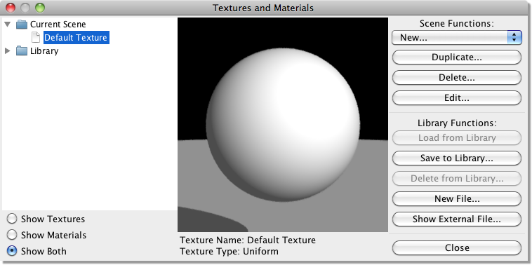
The folders on the left list the textures and Materials in the current scene, as well as those in the texture library that comes with AOI. In the middle of the window is a preview of whichever texture or material is currently selected, and on the right are controls for editing the textures and materials. Most of these are self explanatory. The controls under “Scene Functions” are for working with the textures in the current scene. You can create a new texture, create a duplicate of an existing texture, delete the selected texture, or edit the selected texture. The controls under “Library Functions” are for working with the library. You can copy a texture from the library to the current scene (with Load from Library) or from the current scene to the library (with Save to Library), delete a texture from the library, or add a new file to the library. You also can copy textures between the library and the current scene by dragging them between folders. Show External File is useful for copying textures and materials between files. When you select this command, it prompts you to select an AOI scene, which then appears on the left of the window as if it were part of the built in library.

Once textures have been defined, they can be assigned to any 3-D object and can be mapped in a desirable way by altering their scaling, orientation and position relative to the object. Textures can also be layered to simulate complex real-world surfaces.

7.1. Uniform Textures

Uniform textures are the simplest kind of texture in Art of Illusion. They apply the various surface properties uniformly to the whole object. To create a new uniform texture, Click on Scene -> Textures and select Uniform texture from the New… menu. This will bring up a dialogue box similar to the one below:

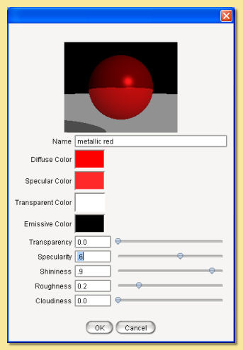
A rendered sphere at the top of the dialogue shows the current texture mapped to a sphere. Double-clicking over the preview will display a pop-up menu as shown below:

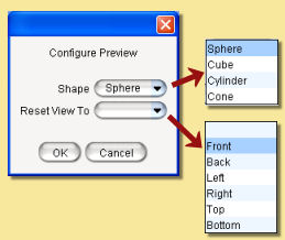
This allows the view to be changed and the 3D object used for the preview to altered.

The preview can also be zoomed via holding CTRL while dragging up and down with the right mouse button and panned by dragging the right mouse button.

Below this are the various properties that can be changed. There are 4 colours that can be defined. Simply click on the colour bar to the right of each colour property. This will bring up the colour chooser dialogue shown below.

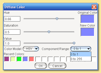
Colours are defined through this dialogue using one of 3 Color Models: Hue, Saturation and Value (HSV), Red, Green and Blue (RGB) or Hue, Saturation and Lightness (HSL). Each colour component can be set to a value according to the selected Component Range (0-1 or 0-255).

Recent colours are also available for selection via the palette at the bottom.

The 4 colour properties are:

Diffuse Colour This is the basic underlying colour of the object. In the absence of any other properties, the object looks this colour.

Specular Colour Specularity is the ‘shininess’ or reflectiveness of the object. The colour specified here defines which colour is reflected by the object. Note, however, that this has no effect unless the specularity value is greater than zero (see below).

Transparent Colour If the transparency of the object is greater than zero, then this colour is that which is transmitted when light passes through the object (see below).

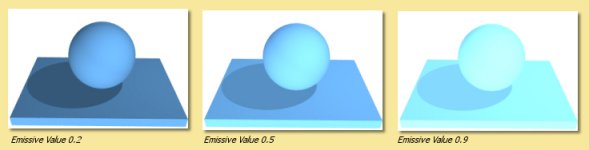
Emissive Colour This property is used to simulate glowing objects. This is the colour that is emitted by the object. Some examples are shown below. In these examples, the Hue and Saturation of the diffuse colour were used for the Emission Colour with varying amounts of Value. Note that the quantity of emitted light is directly related to the Value in the HSV colour, and hence the HSV colour model is probably the most useful for this surface property.

Below the colour properties are 4 numerical quantities with slider bars to define their values.

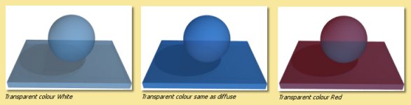
Transparency is the degree to which the object transmits light. A value of 1 means the object is completely transparent and 0 is completely opaque. The images below show objects with a transparency of 0.5. The effect of varying the Transparent Colour is illustated. Normally an transparent object will transmit light of a colour similar to its diffuse colour but in computer graphic imagery we are not limited to physical reality.

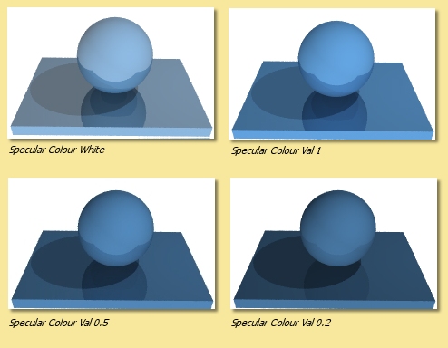
Specularity is the reflectiveness of the object. A value of 1 means the object is completely reflective and thus the diffuse colour will not be visible. A value of 0 is completely non-reflective.

The images on the right show objects all with a specularity of 0.3 and show the effect of varying the Specular Colour.

Plastic type objects normally reflect virtually white light whereas metallic objects tend to reflect light that is tinged with the object’s diffuse colour. In the examples here, the Hue and Saturation of the diffuse colour has been used as the specular colour with varying amounts of Value and compared with a ‘plasticky’ white specularity.

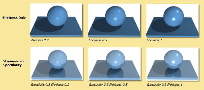
In addition to specularity is Shininess which controls the intensity of specular highlights. Although ‘Shiny’ surfaces in real life are due only to specularity, the shininess parameter is useful to fake some types of effect such as shiny plastic surfaces without much obvious reflection. In most cases, you will want to have both specularity and shininess. Below are examples of different shininess values with and without specularity.

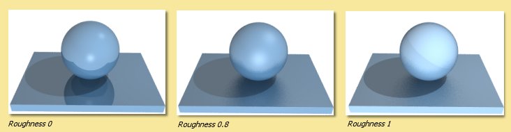
Roughness This parameter can be used to mimic the real life effect that the roughness of a surface decreases the sharpness of reflections. Large Roughness values result in more blurred reflections and more widespread specular highlights as shown below. Note that Gloss/Translucency needs to be enabled during rendering with the raytracing engine (see Rendering) to see the effect.

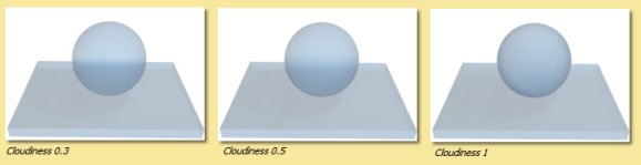
Cloudiness controls the degree of translucency for transparent objects. Higher values cause more blurring of transmitted light as illustrated below. As with the Roughness parameter, Gloss/Translucency needs to be enabled during rendering to see the effect.

7.2. Image Mapped Textures

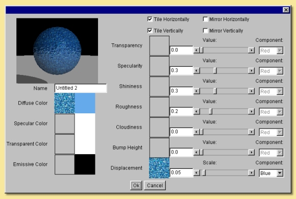
This type of texture allows you to define the surface properties based on 2-D images. These images would usually be created in some 2-D paint program. To create a new image-mapped texture click on Scene->Textures and choose Image Mapped texture from the New… menu. The following dialogue box will be displayed:

The same surface properties as were described in Uniform Textures are also here. This time however, both the colours and the values are determined through the choice of 2-D images. This means that the values of the various parameters vary over the object’s surface according to the image used, instead of being uniform.

On the left of the dialogue box are the diffuse, specular, transparent and emissive colours. If you click on the square box immediately to the right of the text, another dialogue box title ‘Images’ appears. Click Load to read in a new image. The image can be in .jpg, .png, .gif, .svg, or .hdr format. Simply find the image and click on ‘Open’ to get the image. A thumbnail of this image is then displayed in the ‘images’ dialogue box and is automatically selected (shown by being enclosed by a black square). If other images have been read in already then you can select any of them by clicking on them. Once the required image is selected, click on Done. (If you wish to have no image selected, click on Select None).

Note that there is also a uniform colour box next to the image box. The colour specified here modifies the colours of the image map uniformly.

As with the uniform texture dialogue, double-clicking on the preview displays a menu from which the view and preview object can be changed and the preview can be zoomed (CRTL and RMB drag up/down) and panned (RMB drag).

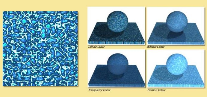
The images below right right show the effect of applying an image map to the various property colours. The image map itself is shown below left:

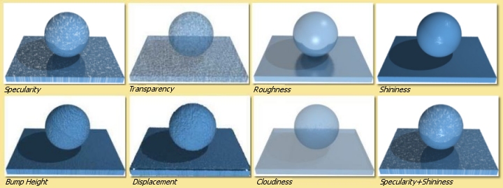
On the right hand side of the image map dialogue are the numerical properties. The properties Transparency, Specularity, Roughness and Cloudiness that were available with Uniform Textures are also here but, in addition, are two different properties; Bump Height and Displacement. These control the ‘bumpiness’ of the surface. Bump mapping varies the surface normals to simulate bumps in the geometry, whereas Displacement mapping actually changes the surface geometry.

For Image Mapped textures, the amount of transparency, specularity etc. is defined by the image map selected by clicking on the square box next to the text. If no image is selected, a uniform value can be specified using the sliders. If an image is selected, the property varies across the surface according to the image. You can choose whether the Red, Green or Blue values are used to control the various parameters by selecting the appropriate Component on the right of the dialogue. For images with information in an alpha channel or which contain transparent regions (of the supported image types, .png, .svg, and .gif support transparency), an additional component named Mask is also available for selection in the component list. This can be used to apply effects to particular parts of the surface only, e.g. only parts of the image within an alpha selection can be made to be shiny etc. The Mask output can also be used to apply surface properties depending on the transparency in the image. The most obvious example would be to use it in the Transparency property where transparent parts of the image would then act as transparent regions in the texture (see example below). However, the mask can be applied in any of the properties for other effects.

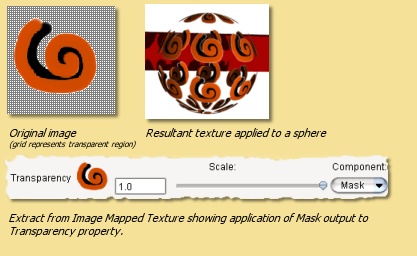
The slider bars then change to control the ‘Scale’ of the effect. In this way, you can make only some parts of the surface transparent, shiny etc. Some examples are shown below:

The image map dialogue also allows you to tile images (on by default) so that the entire surface of the object can be covered if the image is smaller than it and to mirror the image in either axis.

Images used for textures can be managed directly through Scene -> Images. This allows images to be loaded, saved or deleted.

7.3. Procedural Textures

Procedural textures are those in which the various properties described above are defined by mathematical algorithms. There are two types of procedural texture in Art of Illusion: procedural 2D and procedural 3D textures. The 2D textures are essentially thin sheets of texture that are wrapped around the object in a way defined by the mapping (see Assigning Textures). Procedural 3D textures on the other hand are ‘solid’ textures and objects assigned to them will look as if they have been ‘carved’ out of it.

The graphical interface for defining both types of procedural texture are however identical so both will be described in this section.

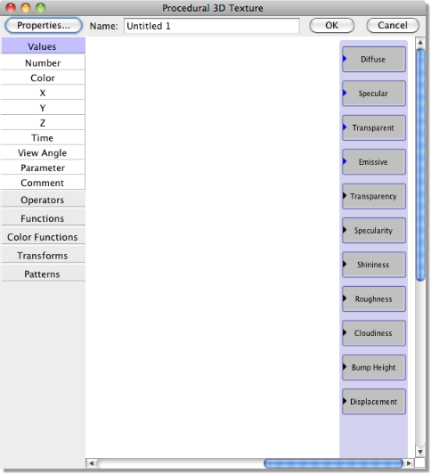
To define a new procedural texture click on Scene -> Textures and choose Procedural 2D texture or Procedural 3D texture from the New… menu. The following window is then displayed:

A preview window is also displayed showing the current texture applied to a sphere.

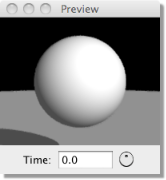
This preview window automatically updates as the texture is built up. The size of this preview can be altered by dragging the sides of the preview window frame and the preview can be zoomed (CTRL drag with RMB) and panned (drag with RMB). As with the uniform texture dialogue, double-clicking on the preview displays a menu from which the view and preview object can be changed.

The preview can also be used to view the texture at a predefined time - useful for textures that vary with time (see example below).

To start with, the preview shows a uniform white texture as this is the default. Please note, however, that 2D textures are shown using projection mapping (link to mapping section), whereas 3D textures are shown using linear mapping. Thus, the same procedural texture might look different for the 2D and 3D preview. All the following examples in this section have been created using 3D procedural textures. As an exercise, you might want to check if they look different for a 2D procedural texture, and if it’s the case, why.

The boxes at the right hand side of the procedural texture editor show the surface texture properties that were described above for the other type of textures. The idea of the procedural texture editor is to pass values (either colours or numbers) into the relevant property boxes. This is done by inserting values, functions and transforms and connecting them to the property boxes. This produces a set of values which are calculated for each point on the surface thus creating the texture.

Along the left side of the window is a menu of ‘modules’ that can be added to the procedure. They are organized into categories, such as Values, Operators, Functions, etc. Click on any category to expand it and see the modules it contains.

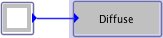
Let’s take a simple example: a uniform diffuse colour. Make sure the Values category is expanded, then click on Color, or alternatively press the mouse on Color and drag onto the blank texture ‘canvas’. A small square appears which looks like . To apply this colour, connect it to the Diffuse colour box by clicking on the blue solid arrow on the end of the ‘color’ box, hold the mouse button down, drag to the blue arrow on the Diffuse box and let go. A line should now be displayed connecting the 2 boxes.

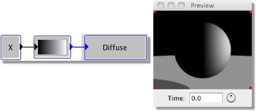
The preview window will be unchanged since the colour in the ‘Color’ box is white by default. Double-click on it and the colour chooser dialogue will be displayed. Select the colour of choice and click on OK. The preview window will now show the new uniform diffuse colour texture.

Each of the values, functions etc. modules selected from the menu has at least one output (shown as arrows pointing outwards) which is either a colour or a number; blue arrows indicate colours, black arrows are numbers. To be precise, the outputs are a set of values representing the colour or value at each point on the surface. Most also have at least one input value which are shown as arrows pointing inwards.

Let’s try something slightly more complicated: a gradient across the surface. Click on the ‘Color’ box and press delete to remove it. This time, click on the Color Functions category to expand it, then drag a Custom module onto the canvas. This produces a colour map.

Connect the output of this to the Diffuse property box. The preview now shows a black sphere. This is because the colour chosen from this colour map depends on the input black solid arrow of this box. If you click and hold on this arrow, you will see that it says Index (0) meaning that the colour map function requires an index and the default for this is 0 which corresponds to black in the colour map. To get a gradient, we need the colour selected from this map to vary according to its spatial position. So, if the gradient is going to run in the X direction, we need to input X to the colour map box. Expand the Values category and insert an X module. The output from this box is the x value of each particular point on the surface. Connect this output to the input of the colour map and the preview window will now show a gradient as shown below:

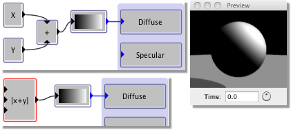
If we had connected a Y box to this, we would have got a gradient in the y-direction. What if we wanted a gradient diagonally? In this case, we need to feed (X+Y) to the input of the color map. Select both X and Y from the Values menu. To perform an addition, we need to insert an Add module from the Operators category. Then connect the outputs of the X and Y boxes to the input arrow of the Add box, and the output of the Add box to the input of the color map as shown on the right:

There is another way we could have achieved this. Under the Functions category is a powerful function called Expression. Select this and double-click on it. This function allows the entry of any mathematical expression of x,y,z, time and the box inputs. Enter ‘x+y’ in the box and click OK. Connect the output of this box to the gradient and the same effect is achieved. This is also shown on the right:

Let’s look now in more detail at the values, functions and transforms available.

Values

This is the Values menu.

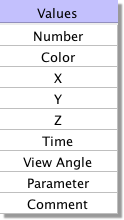
Most of the entries here are self-explanatory:

Number inserts a box with a single constant number. Double-click to change the value.

Color inserts a single constant colour box. Double-click to bring up the colour chooser dialogue to change the colour.

X, Y and Z simply bring up boxes with the x,y,and z values at each point on the surface. For procedural 2D textures, Z is zero.

Time This inserts a box, the output of which is the time value. In animations, this value will change and thus textures, themselves, can be animated.

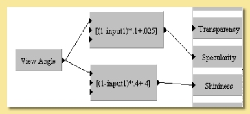
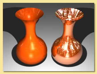
View Angle This module can be used to vary surface properties of an object depending on the angle between the camera and the point on the surface. It has uses in simulating Fresnel effects where the specularity is less at near normal angles of incidence and increases at glancing angles. The View Angle module outputs the Cosine of the angle of incidence and the example below shows how it can be used to generate a Fresnel effect: In this example, the procedural texture shown below left was used to make the left vase more ‘plasticky’ by enhancing reflections at glancing angles. The metallic vase on the right has a higher specularity which is also applied uniformly.

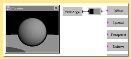
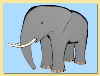
This module has many other uses, one of which is a simple ‘toon’ texture as shown below:

Parameter This allows textures to be dependent on user-defined parameters which can be specified when mapping the texture indivually for objects and even for particular parts of objects. See Texture Parameters for more details.

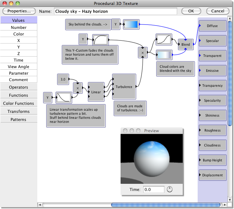
Comment Thus module is purely a text box allowing comments to be placed in the procedure, e.g. to describe parts of the procedure as shown in the example below:

Operators

This is the Operators menu.

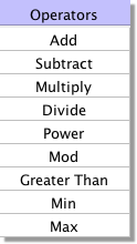
These are standard mathematical operators:

Add, Subtract, Multiply, Divide These boxes each have 2 inputs which are added, subtracted (bottom input from top input),multiplied together or divided (top divided by bottom) depending on the operation selected.

Power The output of this is the left input to the power of the exponent (top input).

Mod has 2 inputs, the dataset to be operated on and a Modulus value. It returns the remainder of dividing the dataset input by the Modulus, e.g if the input was 5 and the Modulus was 4, the output would be the remainder of dividing 5 by 4 which equals 1.

Greater Than returns 1 if the top input is greater than the bottom and 0 otherwise.

Min, Max Both of these have 2 inputs. They are compared and the minimum or maximum respectively is returned as the output.

Functions

This is the Functions menu.

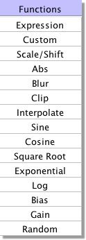
These entries are applied to numerical values to modify them in various ways:

Expression allows the entry of any mathematical expression of x, y, z, t (representing time) and any of 3 inputs to the box. The inputs are identified as input1, input2 and input3.

Expressions can use the following mathematical operations: +,-,/(division),*(multiplication), ^(to the power of),%(modulus) and can contain the following functions: sin(a): sine of a, cos(a): cosine of a, sqrt(a): square root of a, abs(a): absolute value of a, log(a): natural logarithm of a, exp(a): e to the a power (same as e^a), min(a, b): minimum of a and b, max(a, b): maximum of a and b, pow(a, b): a to the b power (same as a^b), angle(a, b): the angle formed by a right triangle with sides a and b, bias(a, b): the Bias function with a bias of b, gain(a, b): the Gain function with a gain of b. The constants, pi and e are also recognised.

Custom allows a curve to be drawn relating the output to the input. New points can be added by clicking on the graph and existing points can be moved by clicking and dragging. The curve can be smoothed by checking the appropriate box. In addition, the function can be made periodic, i.e. it repeats itself forever outside the 0-1 range. Otherwise, input values less than 0 produce the same output as an input of 0 and input values greater than 1 give the same outputs are input values of 1.

Scale/Shift multiplies the input value by a constant value and adds an offset value. Double-click on the box to alter both these values.

Abs returns the absolute value of the input, i.e. if the input is greater than 0, there is no change, if the input is negative, the positive value is returned (e.g. -5 becomes +5).

Blur Produces a blurring effect. There are 2 inputs: one is the set of values that you want to apply the operation to, the other is a value defining the amount of blurring. More accurately, this second value is the range over which the smoothing is performed.

Clip This function limits the input to be within a range specified by double-clicking the box. Input values between the limits are unchanged, values less than the minimum are set equal to the minimum, and inputs greater than the maximum are set equal to the maximum.

Interpolate outputs a value based on 3 inputs. Value 1 and value 2 (top and bottom inputs) specify the maximum and minimum and the fraction input determines the value between the min and max. For example, if the fraction was 0.5, the output would be half-way between the extremes, if it was 0.25, the output would be a quarter of the way between them etc.

Sine, Cosine, Square Root, Exponential, Log These are straightforward mathematical expressions with a single input and output. The inputs for Sine and Cosine are in radians. The Log module is a natural (i.e. to the base e) logarithm.

Bias This module calculates Ken Perlin’s Bias function. Given an input value between 0 and 1, it calculates an output value which is also between 0 and 1 according to: y(x) = x^(log(B)/log(0.5)) where the input value x and bias B correspond to the two input ports. If B=0.5, then y(x)=x. Values of B less than 0.5 push the output toward smaller values, while values of B greater than 0.5 push the output toward larger values.

Gain This module calculates Ken Perlin’s Gain function. Given an input value between 0 and 1, it calculates an output value which is also between 0 and 1 according to: y(x) = Bias(2*x, 1-G)/2 if x-1.5 where the input value x and gain G correspond to the two input ports, and Bias(x, B) is the Bias function described above. If G=0.5, then y(x)=x. Values of G less than 0.5 smooth the input by pushing the output toward 0.5, while values of G greater than 0.5 sharpen the input by pushing the output toward 0 or 1.

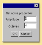
Random This is a one-dimensional random noise pattern. It has 2 inputs, one of which is the dimension over which the random noise is applied and the other is the amount of noise. The input dimension is time by default as this function is most commonly used to vary position/rotation during an animation. This function could, however, be used to create random patterns in space or, indeed, to apply random variations to texture patterns. Also, similarly to some of the Patterns described below, double-clicking the Random module allows the Amplitude and number of Octaves to be specified. See the description of the Noise pattern below for more details of these parameters.

Color Functions

This is the Color Functions menu.

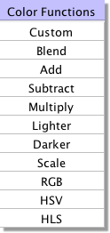
These functions are used to create or change colour values in various ways:

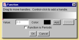
Custom As we have already seen, this is used to creat colour maps from which colours are selected depending on the input numbers. The default colour map has black at one end and white at the other. Double-click on the colour bar box to edit it as shown below. To change a colour, click on the small arrow beneath it on the bar - the arrow will turn red to show it is selected. Then click on the colour square which will display the colour chooser dialogue to enable a new colour to be selected. Colours can be added to the colour map by clicking on Add. This creates a new arrow on the bar which can be coloured as required. The positions of the colour along the bar can be altered either by dragging the arrows to the required place or by entering a number between 0 and 1 into the Value box. The colour map can be made periodic by checking the appropriate box. This means that the colour map repeats itself indefinitely for all points on the surface. If not selected, then parts of the surface outside the map will be a uniform colour the same as the appropriate end of the colour bar.

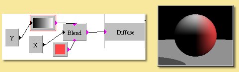
Blend is another way of defining a colour from a range. It takes 2 input colours and blends them according to the numerical input. The important difference between this and the custom colour function is that the colours are inputs are can thus be created by other functions. This is a simple example where one of the colour inputs is a fixed red colour and the other is a colour selected from a custom colour map. The function selecting the colour from the map is simply Y so this would create a gradient in the Y direction. The colour selected and fed into the blend function thus varies from white to black depending on the Y position. This then gets mixed with red according to the X position which is the function fed into the Blend colour function. Obviously much more complicated functions can be defined.

Add, Subtract, Multiply are simple functions that take 2 colour inputs and perform the appropriate mathematical operation on their RGB components.

Lighter, Darker Both these functions take 2 colour inputs and output whichever of the 2 colours is lighter or darker. This is determined by the luminance component of the CIE XYZ color system.

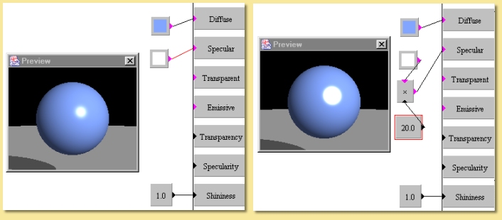
Scale allows the input colour to be scaled by a numerical input. Each component of the input colour is multipled by the input number. One somewhat hidden feature of the colour Scale module is that it can be used to increase properties such as Specularity, Shininess, Transparency etc beyond their normal maximum value of 1. This is done by scaling the appropriate colour (i.e. Specular Color for Specularity and Shininess, Transparent Color for Transparency) by numbers greater than 1. The resulting property value is the product of the scaled colour value and the Number input to the property. An example is shown below: In the left hand image, the Specular Color is white (i.e. Hue-0, Saturation-0 and Value of 1) and the Shininess is set to 1. The overall Shininess is then the product, i.e 1 x 1 = 1. The right hand image uses the Scale module to increase the Specular Color Value to 20; the product is thus 1 x 20 = 20 and the result is a much (artifically) brigher specular highlight which could, for example, be used as a cartoon-like shiny texture.

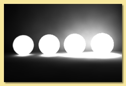
Another use is with emissive textures; the Scale can be used in a similar way to increase the light produced by an emissive object when rendered with Global Illumination. The image below shows the effect of applying the colour Scale module to the Emissive Color; the numerical inputs to the Scale module being 1,2,5 and 10 respectively: The image was rendered with Photon Mapping for Global Illumination.

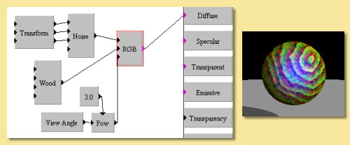
RGB This module allows Red, Green and Blue components to be determined via numerical inputs. is a seemingly simple function, its power lies in the fact that the components are inputs and can therefore be calculated by other function combinations. In the example on the right, the Red component is determined from a Noise module, the Green component is obtained from a Wood pattern and the Blue component is dependent on the View Angle to the Power of 3.

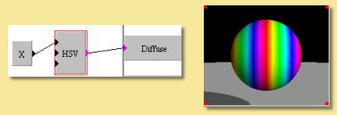
HSV As with the RGB module, this function has 3 numerical inputs; one for each of the colour components. This time the Hue, Saturation and Value components can be controlled via numerical inputs as shown in the simple example on the right in which the Hue is determined by the x-position.

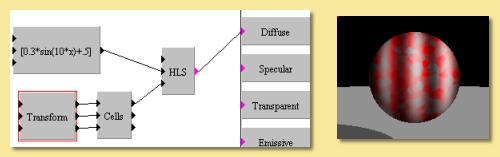
HLS As with the previous two modules, this function has 3 numerical inputs; one for each of the colour components. This time the Hue, Lightness and Saturation components can be controlled as shown on the example on the right in which the Lightness varies sinusoidally and the Saturation is determined from a scaled Cells pattern.

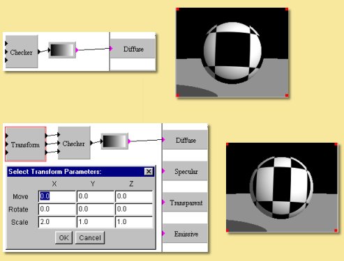
Transforms

The modules in this menu perform transformations on the co-ordinate system. This is the Transforms menu:

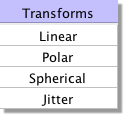
Linear

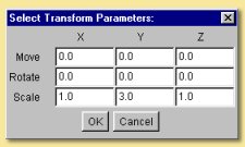
This module allows scaling, rotation and translation of x, y or z. Double-clicking on the box brings up a dialogue allowing entry of the relevant transformation parameters.

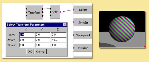
An example is shown below. Here is the same basic texture we had in the HSV example above. The X output of the linear transform is fed into the Hue component of the HSV colour function. With the default transformation settings, this would result in the same texture as before. However, a scaling factor of 5 has been entered in the x column and a 45 degree rotation has been applied in the z-axis to produce the modified texture seen.

Polar

The polar module transforms the linear co-ordinate system of x and y to the polar co-ordinate system defined by r (radial distance) and theta (angle). An example is shown below.

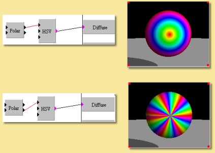
The top example shows the result of feeding the r co-ordinate into the Hue of the HSV function producing a pattern where the colour is the same for points at the same distance from the centre, thereby producing rings of colour.

Similarly with the theta co-ordinate, points at the same angle have the same colour as shown in the lower image.

Spherical

This transforms the linear co-ordinate system to a spherical coordinate system.

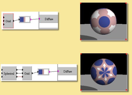
The example below shows an example using the Grid pattern (see below). This is used to select a colour from the custom colour function giving the result in the upper image.

Applying a spherical transfrom to the co-ordinate system before the Grid pattern produces the lower image.

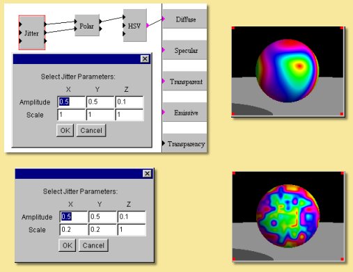
Jitter

This transform keeps a linear co-ordinate system but applies a random jittering effect. Double-clicking on the box displays a dialogue allowing control of the amplitude of the jitter and the range over which the jittering takes place.

In the example below, we have the texture used as an example above under ‘Polar’. This ordinarily produces a set of rings of different colours. This time, however, a jitter has been applied to the x and y co-ordinates of amplitude 0.5. The top image shows the effect with a scale of 1 and the lower image shows what happens when this scale is reduced.

Patterns

There are several pre-defined texture patterns in Art of Illusion accessible through the Patterns menu as shown above. Each pattern has 3 inputs for x, y and z coordinates.

Below we will look at each colour pattern and its variations. In each case, the output from the pattern box has been fed into the default custom colour function and then into the Diffuse property box.

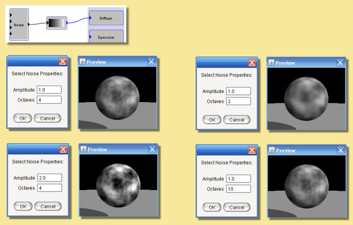
Noise

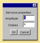
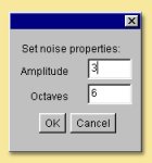
This module creates a fractal noise pattern using Stefan Gustavson’s implementation of Ken Perlin’s Simplex noise function.  For technical details see here. Each octave has twice the frequency of the previous octave. You can specify the number of octaves to use, and the amplitude of the first octave by double-clicking on the noise box. The amplitude of each higher octave is obtained by multiplying the amplitude of the preceding octave by the value of the noise input port (which is typically between 0 and 1, although this is not strictly required). Because this is an input port rather than a parameter, it does not need to be a constant. This is very useful for creating noise patterns whose character varies over the surface of an object.

The noise function is scaled so that output values will typically be between 0 and 1. Depending on the values of the parameters and the noise input, however, the output value may sometimes go outside this range.

Some examples are given below:

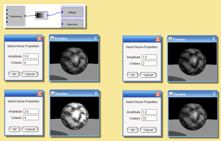
Turbulence

This module is like the Noise module, except that it takes the absolute value of each octave of noise before adding them together. This creates “creases” in the output where its derivative changes discontinuously. The result is somewhat reminiscent of turbulent flows in liquids. The noise function is scaled so that output values will typically be between 0 and 1. Depending on the values of the parameters and the noise input, however, the output value may sometimes be greater than 1.

Some examples are given below:

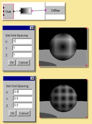
Grid

This module is useful for creating patterns that are based on a uniform grid. It defines a uniform, three dimensional grid of “feature points”. The value at any point is equal to the distance from that point to the nearest feature point. Double-click the module to change the spacing between feature points. Some examples are shown below:

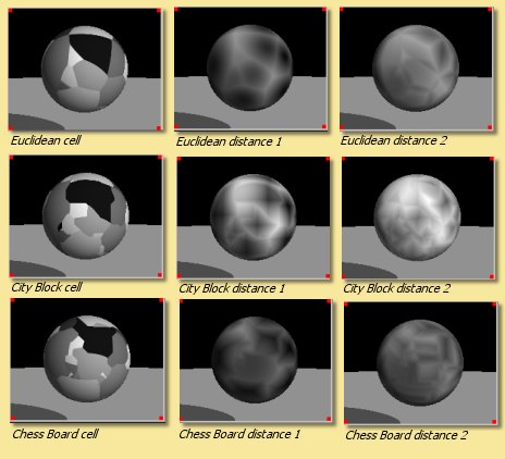
Cells

This texture pattern is similar to the grid function but, instead of the feature points being evenly spaced in a grid, they are positioned randomly. The Cells module box has 3 outputs; The cell port outputs a value between 0 and 1 which identifies the nearest feature point. This value is the same for every point in the “cell” defined by that feature point. This is useful for creating irregularly shaped cells, where each cell is a different color. The distance 1 and distance 2 ports output the distance to the nearest and second nearest feature points, respectively. Distance 1 for the cells pattern is analagous to the grid pattern.

In addition, the distances between each point and the feature points can be calculated using 3 mathematical formula which result in 3 different pattern types; Euclidean, City Block and Chessboard. The type is selected by double-clicking the module box.

The results with each of the 3 outputs and 3 distance types for the default custom colour function are shown below:

The expression distance2-distance1 is a very useful function:

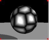
Here, it is plugged into the default custom colour module for the diffuse colour and emissive colour.

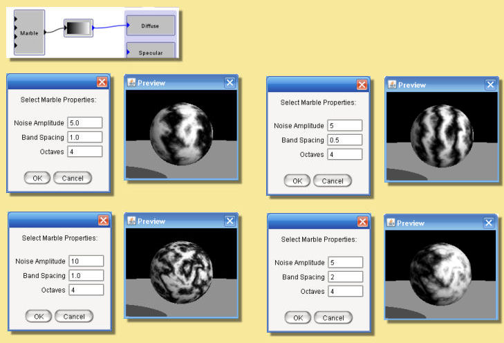
Marble

This is a mathematical pattern that simulates marble. In addition to the x, y and z inputs is a noise input. Double-clicking the module box allows the spacing of the marble bands to be altered as well as the noise amplitude and number of octaves. Some examples are given below:

Wood

Not surprisingly, this pattern is useful for producing wood-like textures. Its output for a given point is proportional to the distance from the Y axis, plus a turbulence function. Double-clicking the Wood module allows the various parameters to be altered; noise amplitude, ring spacing and number of noise octaves. Some examples are given below:

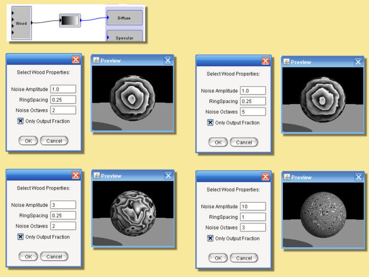
If you select the “Only Output Fraction” option, the output is taken mod 1, so that it consists of a series of concentric rings, with the output increasing from 0 to 1 over the width of each ring. The most common use of this module is to send its output into a Custom color function, which creates an appropriate series of color bands. When used this way, it is generally best not to select the “Only Output Fraction” option, and instead to make the color function periodic. Otherwise, the anti-aliasing of the wood function may lead to visible artifacts.

Checker

This pattern produces the checker board pattern so often seen in 3D computer graphic imagery. There are no options for this pattern but the spacings can be altered by applying scaling to the input x, y and z coordinates:

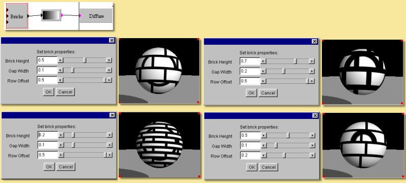
Bricks

This module produces a brick pattern with the ‘bricks’ having an output value of 1 and the ‘mortar’ an output of 0. Double-clicking on the module allows the brick height, gap width and row offset to be varied as shown in the examples below:

Image

This module allows the use of an image within the texture. As with image mapped textures, the image must be in either .gif, .png, .jpg, .svg, or .hdr format. The image module has 5 outputs: a colour map of the image and 4 numerical outputs corresponding to the red, green and blue components and a Mask output which can be used to vary surface properties based on image alpha selections/masks or transparent image regions (see here for more details) .

Double-clicking brings up this dialogue box:

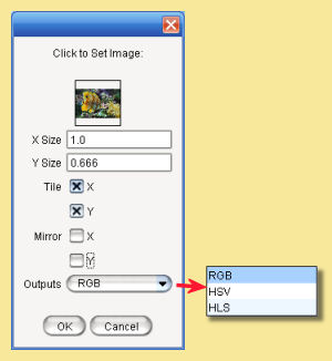
Clicking on the outlined square brings up a dialogue enabling you to select or load an image.

The X-size and Y-size are the relative sizes of the image.

The Tile and Mirror options allow the image to be tiled (simply repeating ad infinitem) in either the x or y direction, or to be mirrored. In the latter case, the images are tiled in such a way that adjacent tiles are mirror images; this allows a seamless blend across the surface.

The Outputs from the module can also be set to either (i) Red, Green & Blue (RGB) (ii) Hue, Saturation & Value (HSV) or (iii) Hue, Lightness & Saturation (HLS).

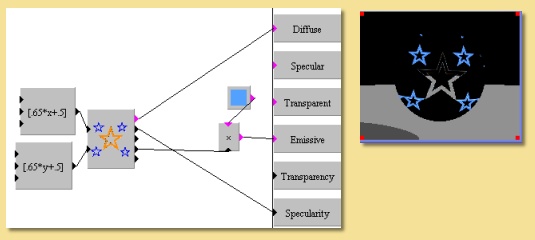
Below is an example of the image module. Because the output has been set to RGB, the outputs from the module are the colour and 4 numerical outputs in the following order: Red, Green, Blue and Mask. Here the blue stars are being given a glow by applying the Blue output of the image module to a Color Scale module which scales a blue Color module input to the Emissive property box. The Red output (which is most prevalent in the orange star) is being used to control the Specularity and the Colour output is a straight input to the Diffuse property.

Edit Menu

The other menu available in the procedural texture editor is the Edit Menu:

Undo/Redo This allows the last action to be undone or redone.

Cut copies the currently selected modules into the clipboard and deletes them from the procedure.

Copy copies the currently selected modules into the clipboard without deleting them.

Paste creates new copies of any modules placed in the clipboard by the Copy and Cut tools.

Clear deletes the currently selected module(s).

Properties This allows the antialiasing of the texture to be altered. Normally the default value of 1 is fine. Values greater than this will cause more smoothing of the texture.

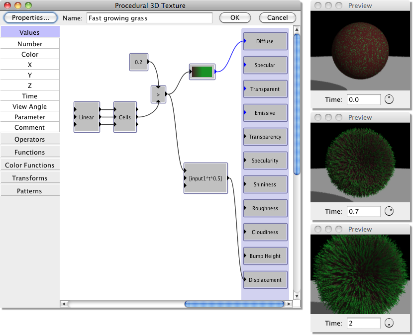
Use of the Preview Time

This image illustrates the use of changing the preview time.

In this example, the height (Displacement) of the ‘grass’ is controlled by the expression input1*t*0.5.  The output of this expression goes from 0 at time (t) = 0, to 0.5 at t=1 secs, 1 at t=2 secs.

Example Procedural Textures

The procedural texture tool is a very powerful way of creating surface textures. The above sections have detailed the various modules available but these only go some way to showing how flexible this approach to textures can be. Most of the modules have been demonstrated only using a simple custom colour map plugged into the diffuse colour property. The modules can however be used to vary any of the colour and number properties and a wide variety of interesting textures can be created.

Here are 3 example textures obtained using a small selection of the available modules in slightly more sophisticated ways. We describe below how each one was created.

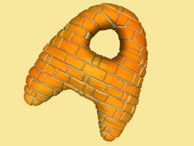
Here is the procedure for the first one:

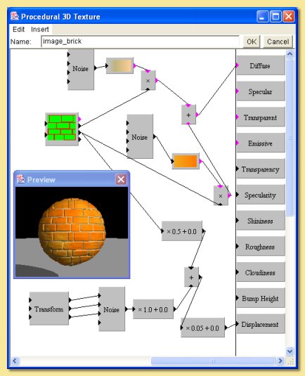
The basis of this texture is a brick-like image consisting of red bricks (R=1,G=0,B=0) and green mortar (R=0,G=1,B=0) as shown below:

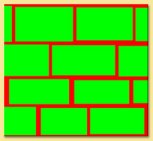
This image is selected with the image pattern module. Because of the way the colours have been used, the green output of this module will have a value of 1 for all green parts of the image (the “bricks”) and 0 for everything else, and the red output will be 1 for all the red parts (the “mortar”) and 0 everywhere else. This enables the bricks and the mortar to have different properties. The red output is multiplied by a noise function (Noise A below) fed into a ‘mortar’ colour map.

This has the result of applying the function only to the mortar. The green output is similarly fed into a brick-like colour map using the noise function (Noise B below).

The two results are summed to give the bricks and the mortar diffuse colour.

We want the bricks to stick out from the surface. This could be simulated using the bump height property but for a more realistic effect, true displacement mapping is used. The green output of the image module has been used to select only the bricks. This has been scaled down by 0.5 and combined with another noise function (Noise C - below) to give an extra random bumpiness. A linear transform (see below) has been applied to scale down this noise in order to add small-scale bumpiness to the bricks.

A further scaling factor of 0.05 has been applied to the combination of brick and noise bumps to reduce the displacement to a more realistic level.

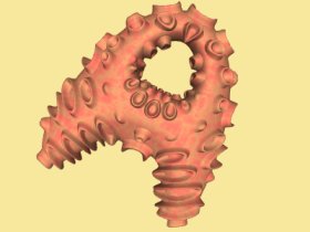
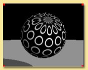
Here is the procedure for the second texture:

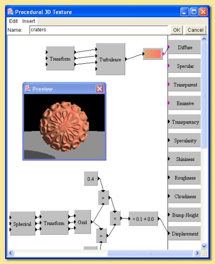
This texture is based around the grid module. With this pattern, the value at any point on the surface is equal to the distance from that point to the nearest ‘feature point’ which are distributed on a grid. The output from the grid module is fed into a greater than function which returns a 1 for any point that is less than 0.4 (i.e. any point within 0.4 units of a feature point) and 0 everywhere else. The grid output is also fed into another greater than function which returns a 1 if the value is greater than 0.3 and 0 everywhere else. The resulting values are multiplied together. Points that had values of 1 for both the greater than functions are the only ones which return a 1, i.e. the overlapping regions which are circular rings. The spherical transform is applied to give spherical symmetry and a linear transformation (scaling 2 in all axes) applied to scale down the pattern. The image below illustrates the result by feeding the output of the multiplication to the default custom colour map into diffuse colour:

Instead of feeding this to the diffuse colour, however, it is used as the input to the displacement property (following a scaling) to give a raised ‘sucker’ effect.

A simple colour function based on the turbulence pattern is plugged into the diffuse colour.

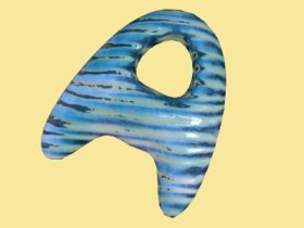
Here is the procedure for the third texture:

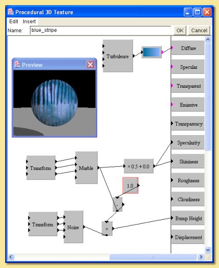
This texture is based on the marble module. This is stretched into a ragged stripe pattern by applying a linear transform (x:2, y:0.1, x:1). The output is scaled and fed into the specularity property causing the stripes to be shiny and the background not.

Small scale bumps are then added only to the not-reflective stripes. The non-reflective stripes are selected by subtracting the marble pattern from 1; this effectively inverses the pattern so that the 1s becomes 0s and vice versa. This is multiplied by the noise pattern used for the bumps so that the bump height is 0 for the reflective stripes.

Finally, a diffuse colour map is created based on the turbulence pattern.